Title: Simple RNA-seq quantification and differential expression pipelines.
Created: 2020-03-18
By: John Urban
For: Anyone interested (Spradling Lab, Carnegie Emb, or otherwise)
Looking at basics of the following programs:
- STAR+RSEM
- Salmon
- HiSat2+StringTie
- EdgeR
- DEseq2
Although this was written up with RNA-seq in mind, much of this can be used for other *-seq and *-ome-wide experiments with or without slight modifications -- e.g. ChIP-seq, ATAC-seq, ribosome profiling, etc.
Below, I describe how to install and use the pertinent software. Importantly, to emphasize that EdgeR and DEseq2 can do much more than independent pairwise analyses between a bunch of samples, I go through doing the DE analysis on an experiment with three time points (T1, T2, T3) with respect to the first time point, T1, or all pairwise comparisons (T1-v-T2, T1-v-T3, T2-v-T3). In my experience, results are more robust when all samples and conditions are analyzed together.
tar -xzf salmon-1.1.0_linux_x86_64.tar.gz
cd STAR/source
make STAR
export PATH=${PATH}:/path/to/STAR/bin/Linux_x86_64
git clone https://github.com/deweylab/RSEM.git
cd RSEM
make
make ebseq
## Change next line for yourself
make install DESTDIR=/mnt/sequence/jurban prefix=/software
unzip hisat2-2.1.0-Linux_x86_64.zip
tar -xzf stringtie-2.1.1.Linux_x86_64.tar.gz
install.packages("BiocManager")
BiocManager::install("pasilla")
BiocManager::install("apeglm")
BiocManager::install("IHW")
BiocManager::install("ashr")
BiocManager::install("vsn")
BiocManager::install("pheatmap")
BiocManager::install("pwr")
BiocManager::install("DESeq2")
BiocManager::install("edgeR")
salmon index -i name -t annotation.fasta
## I used this for paired-end, strand-specific RNA-seq (which was correctly auto-detected by Salmon)
mkdir -p quants
salmon quant -i ${SIDX} -l A \
-1 ${R1} \
-2 ${R2} \
-p 1 --validateMappings -o quants/${PRE}_quant
GFF=/path/to/annotation.gff
RSEM=/path/to/RSEM/rsem-prepare-reference
STAR=/path/to/STAR/bin/Linux_x86_64/
FASTA=/path/to/genome.fasta
${RSEM} --star --star-path ${STAR} --gff3 ${GFF} ${FASTA} star_idx
## This is for paired-end, strand-specific RNA-seq
IDX=/path/to/star_idx
STAR=/path/to/STAR/bin/Linux_x86_64
RSEM=/path/to/RSEM/rsem-calculate-expression
${RSEM} --star --star-path ${STAR} --star-gzipped-read-file --star-output-genome-bam --output-genome-bam --strandedness reverse -p ${P} --paired-end ${R1} ${R2} ${IDX} ${PREFIX} > out.err 2>&1
FASTA=/path/to/genome.fasta
hisat2-build ${FASTA} hisatidx
HIDX=/path/to/hisatidx
STRANDEDNESS=RF
STRINGTIE=/path/to/stringtie-2.1.1.Linux_x86_64/stringtie
GFF=/path/to/annotation.gff
P=1 ## or whatever integer number of threads you have
R1=/path/to/R1.fastq
R2=/path/to/R2.fastq
hisat2 --dta -p ${P} -x ${HIDX} -1 $R1 -2 $R2 --rna-strandness $STRANDEDNESS | samtools sort > reads.bam
mkdir -p ./for_ballgown
${STRINGTIE} --rf -G ${GFF} -e -b ./for_ballgown reads.bam -A ./for_ballgown/gene-level-counts.txt > ./for_ballgown/stringtie.out.gff
# The following command can help make a useful file, but also see output in for_ballgown/:
awk '$1 !~ /^#/ && $3=="transcript" {gsub(/"|;/,""); OFS="\t"; print $12,".",$1,$7,$4,$5,$14,$16,$18,$2}' ./for_ballgown/stringtie.out.gff > transcript-level-counts.txt
Gene_1_isoform_1 118 220 240 207 156 66
Gene_2_isoform_1 8 17 2 2 1 0
Gene_3_isoform_1 4.2 0 0 0 0 0
Gene_4_isoform_1 370.8 839 583 488 316 89
Gene_5_isoform_1 84 218 102 102 68 33
...where c1 and c2 are two different conditions, tissues, or stages.
...and r1, r2, r3 are the replicates for each condition.
To extend upon 2 conditions, though, below I will pretend we have datasets from a time course of 3 time points: T1, T2, T3; with 3 replicates each.
library("DESeq2")
library("IHW")
library("vsn")
library("pheatmap")
library("RColorBrewer")
Depending on your experimental design, there is more than one way to perform DE analysis with EdgeR. Many experimental designs may be the simple A vs B format: treatment vs control, A vs B, time point 1 vs 2. Of course, though, you may want to pursue experimental designs with more than a simple single pairwise comparison: A vs B vs C; T1 vs T2 vs T3; or A,B,C at time points T1,T2,T3. For those, you have at least 3 choices:
1. Analyze each in independent pair-wise fashion (not recommended).
2. Use all of the datasets in the data preparation phase, then analyze each in pairwise fashion, or just the pairwise tests that you're concerned with. (more robust in my opinion/experience).
3. Use all datasets in ANOVA analysis to identify genes that differs between any 2 samples.
Here I will spell out approach #2 as I believe it is most similar to the accompanying DEseq2 analysis, and is what I have found most robust and useful for my purposes. In other words, if you feel overwhelmed at this point by all the options, then just use Approach#2 for now and move on with your life. For Approaches #1 and #3 above, see the end of this blog/document (beyond the DEseq2 section). Note that when you have just the simple pairwise experimental design (A vs B), Approach#2 = Approach#1.
## READ IN COUNTS TABLE
## round() can be used on x as it is below for DEseq2
## BUT it is not necessary, so I don't
x <- read.delim('counts.txt', row.names='index')
x <- x[complete.cases(x),]
## DEFINE GROUPS
group <- factor(c(rep("T1", 3), rep("T2", 3), rep("T3", 3)),
levels = c("T1","T2", T3))
## PREPARE DATA
y <- DGEList(counts=x, group=group)
keep <- filterByExpr(y, min.count = 1, min.total.count=10, min.prop=0.25)
y <- y[keep, , keep.lib.sizes=FALSE]
y <- calcNormFactors(y);
design <- model.matrix(~ 0 + group)
colnames(design) <- levels(group)
y <- estimateDisp(y, design, robust=TRUE)
fit <- glmQLFit(y, design, robust=TRUE)
## CONTRASTS AND DE TESTS
con12 <- makeContrasts(T2 - T1, levels=design)
qlf12 <- glmQLFTest(fit, contrast=con12)
con13 <- makeContrasts(T3 - T1, levels=design)
qlf13 <- glmQLFTest(fit, contrast=con13)
con23 <- makeContrasts(T3 - T2, levels=design)
qlf23 <- glmQLFTest(fit, contrast=con23)
## FINALIZING
## I add Benjamini-Hochberg adjusted p-values, and the -log10 versions of each before writing out to a text file.
## E.g. for QLF in [qlf12, qlf13, qlf23]; do this:
## More and more, I have been doing all follow-up analyses in Jupyter Notebooks with Python3 rather than RStudio
## GET BH FDR
fdr <- p.adjust(QLF$PValue, method="BH")
## WRITE OUT
write.table(
x = data.frame(names=rownames(QLF),
QLF,
fdr = fdr,
log10p = -log10(df$PValue),
log10fdr = -log10(fdr)),
file = out,
quote = FALSE,
row.names = FALSE,
sep = "\t")
I will show how to. create a dataframe and output table that includes all 4 logFC estimates, the p-value and FDR from the original statistical tests, and the additional S values from ashr and apeglm. One can then mess around with exploratory analyses comparing these approaches anyway one sees fit.
This approach will only give the comparisons analogous to EdgeR's "T2 - T1" and
"T3 - T1" above.
## READ IN COUNTS TABLE
## Expected counts from RSEM or Salmon can be non-integer (e.g. 4000.245)
## DEseq2 wants integers though.
## round() is used here to convert to the nearest integer value.
x <- read.delim('counts.txt', row.names='index')
x <- round( x[complete.cases(x),] )
## FACTORS
group <- factor(c(rep("T1", 3), rep("T2", 3), rep("T3", 3)),
levels = c("T1","T2", T3))
coldata <- data.frame(condition=group, row.names = colnames(cts))
## DEseq OBJ INITIATE
dds <- DESeqDataSetFromMatrix(countData = cts,
colData = coldata,
design = ~ condition)
## FILTER similar to EdgeR (change as you see fit)
keep <- rowSums(counts(dds)) >= 10 & (rowSums(counts(dds) >= 1)/rowSums(counts(dds) >= 0) >=0.4)
dds <- dds[keep,]
## DIFF EXP ANALYSIS
dds <- DESeq(dds)
## OUTPUTS:
system("mkdir -p deseqtables")
pfx <- "deseqtables/"
pwgrps <- resultsNames(dds)
ngrps <- length(pwgrps) ## idx1 is Intercept
for (i in 2:ngrps){
grp <- pwgrps[i]
print(grp)
splt <- strsplit(grp, split = "_")[[1]]
res <- results(dds,contrast=c(splt[1], splt[2], splt[4]))
resLFC.deseq22014 <- lfcShrink(dds, coef=grp, type="normal")[,2:3]
resLFC.ashr2016 <- lfcShrink(dds, coef=grp, type="ashr", svalue=TRUE)[,2:4]
resLFC.apeglm2018 <- lfcShrink(dds, coef=grp, type="apeglm",svalue=TRUE)[,2:4]
a12 <- merge(as.data.frame(res), as.data.frame(resLFC.deseq22014), by=0, suffix=c("",".shrink"))
a12 <- as.data.frame(a12[,2:dim(a12)[2]],row.names = a12[,1])
a34 <- merge(as.data.frame(resLFC.ashr2016), as.data.frame(resLFC.apeglm2018), by=0, suffix=c(".ashr",".apeglm"))
a34 <- as.data.frame(a34[,2:dim(a34)[2]],row.names = a34[,1])
a1234 <- merge(a12, a34, by=0)
a1234 <- as.data.frame(a1234[,2:dim(a1234)[2]],row.names = a1234[,1])
sfx <- paste0("-", splt[2], "_", splt[4], ".txt")
writeDEseq(df = a1234,
out = paste0(pfx, outpre, sfx))
}
## DEFINE GROUPS
group <- factor(c(rep("T1", 3), rep("T2", 3), rep("T3", 3)),
levels = c("T1","T2", T3))
## PREPARE DATA
y <- DGEList(counts=x, group=group)
keep <- filterByExpr(y, min.count = 1, min.total.count=10, min.prop=0.25)
y <- y[keep, , keep.lib.sizes=FALSE]
y <- calcNormFactors(y);
design <- model.matrix(~ 0 + group)
colnames(design) <- levels(group)
y <- estimateDisp(y, design, robust=TRUE)
fit <- glmQLFit(y, design, robust=TRUE)
## SINGLE CONTRAST AND DE TEST LINE
conAnova <- makeContrasts(
T1T2 = T2 - T1,
T1T2 = T3 - T1,
T2T3 = T3 - T2,
levels=design)
anov <- glmQLFTest(fit, contrast=conAnova)
FDR_anova <- p.adjust(anov$table$PValue, method="BH");
## Read in counts or expected counts table
f <- '/path/to/counts.txt'
x <- read.delim(f, row.names='index')
x <- x[complete.cases(x),]
x12 <- x[,c(1:3, 4:6)];
x13 <- x[,c(1:3, 7:9)];
x23 <- x[,c(4:6, 7:9)];
## Define groups
group12 <- factor(c(rep("T1", 3), rep("T2", 3),
levels = c("T1","T2"))
group13 <- factor(c(rep("T1", 3), rep("T3", 3),
levels = c("T1","T3"))
group23 <- factor(c(rep("T2", 3), rep("T3", 3),
levels = c("T2","T3"))
y12 <- DGEList(counts=x12, group=group12)
y13 <- DGEList(counts=x13, group=group13)
y23 <- DGEList(counts=x23, group=group23)
keep12 <- filterByExpr(y12, min.count = 1, min.total.count=10, min.prop=0.25)
keep13 <- filterByExpr(y13, min.count = 1, min.total.count=10, min.prop=0.25)
keep23 <- filterByExpr(y23, min.count = 1, min.total.count=10, min.prop=0.25)
y12 <- y12[keep12, , keep.lib.sizes=FALSE]
y13 <- y13[keep13, , keep.lib.sizes=FALSE]
y23 <- y23[keep23, , keep.lib.sizes=FALSE]
y12 <- calcNormFactors(y12)
y13 <- calcNormFactors(y13)
y23 <- calcNormFactors(y23)
design12 <- model.matrix(~ 0 + group12)
design13 <- model.matrix(~ 0 + group13)
design23 <- model.matrix(~ 0 + group23)
colnames(design12) <- levels(group12)
colnames(design13) <- levels(group13)
colnames(design23) <- levels(group23)
y12 <- estimateDisp(y12, design12, robust=TRUE)
y13 <- estimateDisp(y13, design13, robust=TRUE)
y23 <- estimateDisp(y23, design23, robust=TRUE)
fit12 <- glmQLFit(y12, design12, robust=TRUE)
fit13 <- glmQLFit(y13, design13, robust=TRUE)
fit23 <- glmQLFit(y23, design23, robust=TRUE)
con12.pw <- makeContrasts(T2 - T1, levels=design12)
con13.pw <- makeContrasts(T3 - T1, levels=design13)
con23.pw <- makeContrasts(T3 - T2, levels=design23)
qlf12.pw <- glmQLFTest(fit12, contrast=con12.pw)
qlf13.pw <- glmQLFTest(fit13, contrast=con13.pw)
qlf23.pw <- glmQLFTest(fit23, contrast=con23.pw)
FDR_12.pw <- p.adjust(qlf12.pw$table$PValue, method="BH")
FDR_13.pw <- p.adjust(qlf13.pw$table$PValue, method="BH")
FDR_23.pw <- p.adjust(qlf23.pw$table$PValue, method="BH")


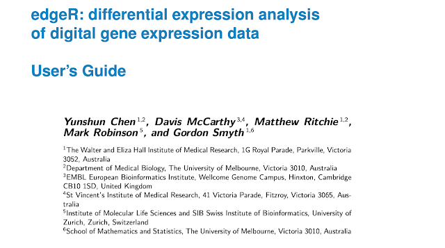
The User's Guide explains the inner workings well, and has all other pertinent references (image below, but no links):


The 'apeglm' adaptive shrinkage estimator:


From sleuth paper:
1. "....sleuth displayed higher sensitivity than Cuffdiff 2, DESeq, DESeq2, EBSeq, edgeR, voom...."
2. "Our results show that by accounting for uncertainty in quantifications, sleuth is more accurate than previous approaches at both the gene and isoform levels. Crucially, the estimated FDRs reported by sleuth are well controlled and reflect the true FDRs, making the predictions of sleuth reliable and useful in practice."
- STAR+RSEM
- Salmon
- HiSat2+StringTie
- EdgeR
- DEseq2
Although this was written up with RNA-seq in mind, much of this can be used for other *-seq and *-ome-wide experiments with or without slight modifications -- e.g. ChIP-seq, ATAC-seq, ribosome profiling, etc.
Below, I describe how to install and use the pertinent software. Importantly, to emphasize that EdgeR and DEseq2 can do much more than independent pairwise analyses between a bunch of samples, I go through doing the DE analysis on an experiment with three time points (T1, T2, T3) with respect to the first time point, T1, or all pairwise comparisons (T1-v-T2, T1-v-T3, T2-v-T3). In my experience, results are more robust when all samples and conditions are analyzed together.
Installation:
Salmon:
wget https://github.com/COMBINE-lab/salmon/releases/download/v1.1.0/salmon-1.1.0_linux_x86_64.tar.gztar -xzf salmon-1.1.0_linux_x86_64.tar.gz
Star:
git clone https://github.com/alexdobin/STAR.gitcd STAR/source
make STAR
RSEM:
## Change next line for yourselfexport PATH=${PATH}:/path/to/STAR/bin/Linux_x86_64
git clone https://github.com/deweylab/RSEM.git
cd RSEM
make
make ebseq
## Change next line for yourself
make install DESTDIR=/mnt/sequence/jurban prefix=/software
HiSat2:
wget http://ccb.jhu.edu/software/hisat2/dl/hisat2-2.1.0-Linux_x86_64.zipunzip hisat2-2.1.0-Linux_x86_64.zip
StringTie:
wget http://ccb.jhu.edu/software/stringtie/dl/stringtie-2.1.1.Linux_x86_64.tar.gztar -xzf stringtie-2.1.1.Linux_x86_64.tar.gz
EdgeR and DEseq2 (in RStudio):
## I am also adding in some dependencies and/or extensions (mostly for DEseq2 uses)
if (!requireNamespace("BiocManager", quietly = TRUE))install.packages("BiocManager")
BiocManager::install("pasilla")
BiocManager::install("apeglm")
BiocManager::install("IHW")
BiocManager::install("ashr")
BiocManager::install("vsn")
BiocManager::install("pheatmap")
BiocManager::install("pwr")
BiocManager::install("DESeq2")
BiocManager::install("edgeR")
Basic Quantification Pipeline Commands:
Salmon:
https://combine-lab.github.io/salmon/Indexing:
https://combine-lab.github.io/salmon/getting_started/#indexing-txomesalmon index -i name -t annotation.fasta
Quantification:
https://combine-lab.github.io/salmon/getting_started/#quantifying-samples## I used this for paired-end, strand-specific RNA-seq (which was correctly auto-detected by Salmon)
mkdir -p quants
salmon quant -i ${SIDX} -l A \
-1 ${R1} \
-2 ${R2} \
-p 1 --validateMappings -o quants/${PRE}_quant
STAR+RSEM:
http://deweylab.biostat.wisc.edu/rsem/rsem-calculate-expression.htmlIndexing:
GFF=/path/to/annotation.gff
RSEM=/path/to/RSEM/rsem-prepare-reference
STAR=/path/to/STAR/bin/Linux_x86_64/
FASTA=/path/to/genome.fasta
${RSEM} --star --star-path ${STAR} --gff3 ${GFF} ${FASTA} star_idx
Quantification:
## This is for paired-end, strand-specific RNA-seq
IDX=/path/to/star_idx
STAR=/path/to/STAR/bin/Linux_x86_64
RSEM=/path/to/RSEM/rsem-calculate-expression
${RSEM} --star --star-path ${STAR} --star-gzipped-read-file --star-output-genome-bam --output-genome-bam --strandedness reverse -p ${P} --paired-end ${R1} ${R2} ${IDX} ${PREFIX} > out.err 2>&1
HiSat2+StringTie:
Indexing:
FASTA=/path/to/genome.fasta
hisat2-build ${FASTA} hisatidx
Quantification:
## This is for paired-end, strand-specific RNA-seqHIDX=/path/to/hisatidx
STRANDEDNESS=RF
STRINGTIE=/path/to/stringtie-2.1.1.Linux_x86_64/stringtie
GFF=/path/to/annotation.gff
P=1 ## or whatever integer number of threads you have
R1=/path/to/R1.fastq
R2=/path/to/R2.fastq
hisat2 --dta -p ${P} -x ${HIDX} -1 $R1 -2 $R2 --rna-strandness $STRANDEDNESS | samtools sort > reads.bam
mkdir -p ./for_ballgown
${STRINGTIE} --rf -G ${GFF} -e -b ./for_ballgown reads.bam -A ./for_ballgown/gene-level-counts.txt > ./for_ballgown/stringtie.out.gff
# The following command can help make a useful file, but also see output in for_ballgown/:
awk '$1 !~ /^#/ && $3=="transcript" {gsub(/"|;/,""); OFS="\t"; print $12,".",$1,$7,$4,$5,$14,$16,$18,$2}' ./for_ballgown/stringtie.out.gff > transcript-level-counts.txt
Basic Differential Expression Commands:
Getting started:
Both EdgeR and DEseq2 analyses can be done in RStudio.
Get your tab-separated counts or expected counts table (counts.txt) set up as such:
index c1_r1 c1_r2 c1_r3 c2_r1 c2_r2 c2_r3Gene_1_isoform_1 118 220 240 207 156 66
Gene_2_isoform_1 8 17 2 2 1 0
Gene_3_isoform_1 4.2 0 0 0 0 0
Gene_4_isoform_1 370.8 839 583 488 316 89
Gene_5_isoform_1 84 218 102 102 68 33
...where c1 and c2 are two different conditions, tissues, or stages.
...and r1, r2, r3 are the replicates for each condition.
To extend upon 2 conditions, though, below I will pretend we have datasets from a time course of 3 time points: T1, T2, T3; with 3 replicates each.
Load needed libraries:
library("edgeR")library("DESeq2")
library("IHW")
library("vsn")
library("pheatmap")
library("RColorBrewer")
EdgeR:
Depending on your experimental design, there is more than one way to perform DE analysis with EdgeR. Many experimental designs may be the simple A vs B format: treatment vs control, A vs B, time point 1 vs 2. Of course, though, you may want to pursue experimental designs with more than a simple single pairwise comparison: A vs B vs C; T1 vs T2 vs T3; or A,B,C at time points T1,T2,T3. For those, you have at least 3 choices:
1. Analyze each in independent pair-wise fashion (not recommended).
2. Use all of the datasets in the data preparation phase, then analyze each in pairwise fashion, or just the pairwise tests that you're concerned with. (more robust in my opinion/experience).
3. Use all datasets in ANOVA analysis to identify genes that differs between any 2 samples.
Here I will spell out approach #2 as I believe it is most similar to the accompanying DEseq2 analysis, and is what I have found most robust and useful for my purposes. In other words, if you feel overwhelmed at this point by all the options, then just use Approach#2 for now and move on with your life. For Approaches #1 and #3 above, see the end of this blog/document (beyond the DEseq2 section). Note that when you have just the simple pairwise experimental design (A vs B), Approach#2 = Approach#1.
## READ IN COUNTS TABLE
## round() can be used on x as it is below for DEseq2
## BUT it is not necessary, so I don't
x <- read.delim('counts.txt', row.names='index')
x <- x[complete.cases(x),]
## DEFINE GROUPS
group <- factor(c(rep("T1", 3), rep("T2", 3), rep("T3", 3)),
levels = c("T1","T2", T3))
## PREPARE DATA
y <- DGEList(counts=x, group=group)
keep <- filterByExpr(y, min.count = 1, min.total.count=10, min.prop=0.25)
y <- y[keep, , keep.lib.sizes=FALSE]
y <- calcNormFactors(y);
design <- model.matrix(~ 0 + group)
colnames(design) <- levels(group)
y <- estimateDisp(y, design, robust=TRUE)
fit <- glmQLFit(y, design, robust=TRUE)
## CONTRASTS AND DE TESTS
con12 <- makeContrasts(T2 - T1, levels=design)
qlf12 <- glmQLFTest(fit, contrast=con12)
con13 <- makeContrasts(T3 - T1, levels=design)
qlf13 <- glmQLFTest(fit, contrast=con13)
con23 <- makeContrasts(T3 - T2, levels=design)
qlf23 <- glmQLFTest(fit, contrast=con23)
## FINALIZING
## I add Benjamini-Hochberg adjusted p-values, and the -log10 versions of each before writing out to a text file.
## E.g. for QLF in [qlf12, qlf13, qlf23]; do this:
## More and more, I have been doing all follow-up analyses in Jupyter Notebooks with Python3 rather than RStudio
## GET BH FDR
fdr <- p.adjust(QLF$PValue, method="BH")
## WRITE OUT
write.table(
x = data.frame(names=rownames(QLF),
QLF,
fdr = fdr,
log10p = -log10(df$PValue),
log10fdr = -log10(fdr)),
file = out,
quote = FALSE,
row.names = FALSE,
sep = "\t")
DEseq2:
DEseq2 has 4 ways to look at the Log2-fold-change estimates. These differences are not part of the DE tests, they are used to have potentially-more-useful visualizations and rankings based on log2FC (that can often be more extreme and error-prone for lower-abundance transcripts).
The 4 ways are:
1. Default log2FC as seen before any shrinkage
2. The original DEseq2 shrinkage from their 2014 paper ("normal" option in lfcShrink())
3. The ashr approach from a 2016-2017 paper ('ashr')
4. The apeglm approach from their 2018-2019 paper ('apeglm')
The latter two (ashr and apeglm), and specifically the last one (apeglm), are recommended by the DEseq2 authors for visualization and ranking. In other words: too many options? confused? Just use apeglm for ranking (i.e. to select top 50 genes) and visualization (e.g in MA plots, Volcano plots) and move on with your life.
The latter 2 approaches (ashr and apeglm) also gives "S values".
The latter 2 approaches (ashr and apeglm) also gives "S values".
From the lfcShrink help:
"The s-values returned in combination with apeglm provide the probability of FSOS events, "false sign or small", among the tests with equal or smaller s-value than a given gene's s-value, where "small" is specified by lfcThreshold."
and
"s-values provide the probability of false signs among the tests with equal or smaller s-value than a given given's s-value. See Stephens (2016) reference on s-values."
This approach will only give the comparisons analogous to EdgeR's "T2 - T1" and
"T3 - T1" above.
## READ IN COUNTS TABLE
## Expected counts from RSEM or Salmon can be non-integer (e.g. 4000.245)
## DEseq2 wants integers though.
## round() is used here to convert to the nearest integer value.
x <- read.delim('counts.txt', row.names='index')
x <- round( x[complete.cases(x),] )
## FACTORS
group <- factor(c(rep("T1", 3), rep("T2", 3), rep("T3", 3)),
levels = c("T1","T2", T3))
coldata <- data.frame(condition=group, row.names = colnames(cts))
## DEseq OBJ INITIATE
dds <- DESeqDataSetFromMatrix(countData = cts,
colData = coldata,
design = ~ condition)
## FILTER similar to EdgeR (change as you see fit)
keep <- rowSums(counts(dds)) >= 10 & (rowSums(counts(dds) >= 1)/rowSums(counts(dds) >= 0) >=0.4)
dds <- dds[keep,]
## DIFF EXP ANALYSIS
dds <- DESeq(dds)
## OUTPUTS:
system("mkdir -p deseqtables")
pfx <- "deseqtables/"
pwgrps <- resultsNames(dds)
ngrps <- length(pwgrps) ## idx1 is Intercept
for (i in 2:ngrps){
grp <- pwgrps[i]
print(grp)
splt <- strsplit(grp, split = "_")[[1]]
res <- results(dds,contrast=c(splt[1], splt[2], splt[4]))
resLFC.deseq22014 <- lfcShrink(dds, coef=grp, type="normal")[,2:3]
resLFC.ashr2016 <- lfcShrink(dds, coef=grp, type="ashr", svalue=TRUE)[,2:4]
resLFC.apeglm2018 <- lfcShrink(dds, coef=grp, type="apeglm",svalue=TRUE)[,2:4]
a12 <- merge(as.data.frame(res), as.data.frame(resLFC.deseq22014), by=0, suffix=c("",".shrink"))
a12 <- as.data.frame(a12[,2:dim(a12)[2]],row.names = a12[,1])
a34 <- merge(as.data.frame(resLFC.ashr2016), as.data.frame(resLFC.apeglm2018), by=0, suffix=c(".ashr",".apeglm"))
a34 <- as.data.frame(a34[,2:dim(a34)[2]],row.names = a34[,1])
a1234 <- merge(a12, a34, by=0)
a1234 <- as.data.frame(a1234[,2:dim(a1234)[2]],row.names = a1234[,1])
sfx <- paste0("-", splt[2], "_", splt[4], ".txt")
writeDEseq(df = a1234,
out = paste0(pfx, outpre, sfx))
}
EdgeR ALTERNATIVE APPROACHES:
ANOVA APPROACH:
## DEFINE GROUPS
group <- factor(c(rep("T1", 3), rep("T2", 3), rep("T3", 3)),
levels = c("T1","T2", T3))
## PREPARE DATA
y <- DGEList(counts=x, group=group)
keep <- filterByExpr(y, min.count = 1, min.total.count=10, min.prop=0.25)
y <- y[keep, , keep.lib.sizes=FALSE]
y <- calcNormFactors(y);
design <- model.matrix(~ 0 + group)
colnames(design) <- levels(group)
y <- estimateDisp(y, design, robust=TRUE)
fit <- glmQLFit(y, design, robust=TRUE)
## SINGLE CONTRAST AND DE TEST LINE
conAnova <- makeContrasts(
T1T2 = T2 - T1,
T1T2 = T3 - T1,
T2T3 = T3 - T2,
levels=design)
anov <- glmQLFTest(fit, contrast=conAnova)
FDR_anova <- p.adjust(anov$table$PValue, method="BH");
INDEPENDENT PAIRWISE APPROACH:
## This can be simply automated in a function and/or for loop, but I spell out everything below in case it is simpler to follow.## Read in counts or expected counts table
f <- '/path/to/counts.txt'
x <- read.delim(f, row.names='index')
x <- x[complete.cases(x),]
x12 <- x[,c(1:3, 4:6)];
x13 <- x[,c(1:3, 7:9)];
x23 <- x[,c(4:6, 7:9)];
## Define groups
group12 <- factor(c(rep("T1", 3), rep("T2", 3),
levels = c("T1","T2"))
group13 <- factor(c(rep("T1", 3), rep("T3", 3),
levels = c("T1","T3"))
group23 <- factor(c(rep("T2", 3), rep("T3", 3),
levels = c("T2","T3"))
y12 <- DGEList(counts=x12, group=group12)
y13 <- DGEList(counts=x13, group=group13)
y23 <- DGEList(counts=x23, group=group23)
keep12 <- filterByExpr(y12, min.count = 1, min.total.count=10, min.prop=0.25)
keep13 <- filterByExpr(y13, min.count = 1, min.total.count=10, min.prop=0.25)
keep23 <- filterByExpr(y23, min.count = 1, min.total.count=10, min.prop=0.25)
y12 <- y12[keep12, , keep.lib.sizes=FALSE]
y13 <- y13[keep13, , keep.lib.sizes=FALSE]
y23 <- y23[keep23, , keep.lib.sizes=FALSE]
y12 <- calcNormFactors(y12)
y13 <- calcNormFactors(y13)
y23 <- calcNormFactors(y23)
design12 <- model.matrix(~ 0 + group12)
design13 <- model.matrix(~ 0 + group13)
design23 <- model.matrix(~ 0 + group23)
colnames(design12) <- levels(group12)
colnames(design13) <- levels(group13)
colnames(design23) <- levels(group23)
y12 <- estimateDisp(y12, design12, robust=TRUE)
y13 <- estimateDisp(y13, design13, robust=TRUE)
y23 <- estimateDisp(y23, design23, robust=TRUE)
fit12 <- glmQLFit(y12, design12, robust=TRUE)
fit13 <- glmQLFit(y13, design13, robust=TRUE)
fit23 <- glmQLFit(y23, design23, robust=TRUE)
con12.pw <- makeContrasts(T2 - T1, levels=design12)
con13.pw <- makeContrasts(T3 - T1, levels=design13)
con23.pw <- makeContrasts(T3 - T2, levels=design23)
qlf12.pw <- glmQLFTest(fit12, contrast=con12.pw)
qlf13.pw <- glmQLFTest(fit13, contrast=con13.pw)
qlf23.pw <- glmQLFTest(fit23, contrast=con23.pw)
FDR_12.pw <- p.adjust(qlf12.pw$table$PValue, method="BH")
FDR_13.pw <- p.adjust(qlf13.pw$table$PValue, method="BH")
FDR_23.pw <- p.adjust(qlf23.pw$table$PValue, method="BH")
Some additional thoughts:
RNA-seq
Overall, for most people and most RNA-seq analyses I recommend:
1. Salmon or Kallisto:
Salmon is just so easy to use, so fast and light weight. It is my understanding that the same can be said for Kallisto, and that these 2 programs produce essentially the same results.
See this blog by the PI behind Kallisto:
It made me feel slightly bad for arbitrarily choosing to use Salmon first, but c'est la vie.
2. STAR+RSEM:
This may still slightly outperform Salmon and Kallisto, although I wouldn't be surprised if I was wrong on that.
Differential abundance/enrichment:
I don't have an opinion yet on whether EdgeR or DEseq2 is better. Perhaps neither is "better".
It appears to me that they have a lot in common, and in my hands give similar results.
Each is often considered the "best" in DE bake-off papers -- and often they are tied.
Both can handle some really complex experimental designs.
- e.g. time courses
- e.g. time courses with different drug treatments
- e.g. experiments where some samples were single-end, others were paired-end
- e.g. analyses using datasets from different labs
In the more complex cases above, these programs can identify batch effects and effects due to differences like SE vs PE reads.
As a result, it can remove those systematic biases and tell you the genes/transcripts/bins that differ due only to biological effects.
EdgeR has an ANOVA option for complex experiments as well.
DEseq2 has some very cool log2FC shrinkage options for visualization and ranking.
It might be worth your time to get familiar with each.
For ChIP-seq, ATAC-seq, and other DNA approaches:
1. Bowtie2 + RSEM
2. I am very interested in trying Salmon or Kallisto on genomic bins (e.g. bin sizes of 50 bp, 100 bp, 500 bp, 1 kb or X... depending on sequencing depth).
For tried-and-true, stick with #1.
For exploratory purposes, mess around with #2.
I foresee #1 being better than #2, though, b/c the EM steps in #2 would be treating genomic bins independently. This hypothetically could be an issue since neighboring bins clearly would have pertinent information for the EM ML estimates. In contrast, RSEM is likely not confined to discrete fixed bins. It is more likely that RSEM can gather information in a bin around each given read -- i.e. the bins are not fixed with reads potentially mapping within them, the read positions are fixed with bins formed around them. Perhaps a kind or hyper-critical reader will comment on that. Nevertheless, perhaps this hypothetical issue is not a big issue in practice, or perhaps it could simply finding the "best" kmer-size for Salmon/Kallisto would overcome this in your particular genomic anakysis. Or perhaps one could use overlapping windows (e.g. bin-size 100, step-size 20) to obtain the ML estimates, followed by taking the average or median within intersecting regions. That could incorporate information from neighboring bins.
I definitely recommend using EdgeR or DEseq2 to do between-sample comparisons for DNA-seq experiments, at least to get the appropriate normalized counts between treatment and controls. In practice, often times one can get away with a simple MACS2 analysis, but EdgeR and DEseq2 seem a bit more principled to me.
References and Resources:
Click images to go to PubMed page for given paper.
Alignment:
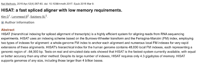
HiSat2:
STAR:
Quantification:
RSEM:
Salmon:
Kallisto:
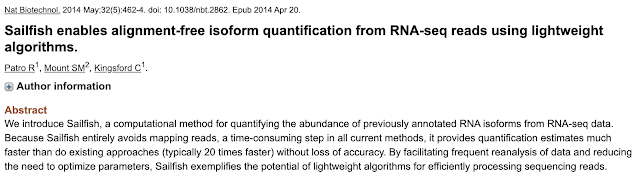
SailFish:
StringTie:
Differential Expression Analysis:
Differential Naming Analysis:
- Differential abundance analysis
- Differential counts analysis
- Differential frequency analysis
- Differential level analysis
- Differential enrichment analysis
- Etc
EdgeR, including the pre-cursor, primary, and follow-up/update papers and resources:
The User's Guide explains the inner workings well, and has all other pertinent references (image below, but no links):


DEseq2, including the pre-cursor, primary, and follow-up/update papers and resources:
The 'ashr' adaptive shrinkage estimator:
The 'apeglm' adaptive shrinkage estimator:
sleuth (penalties incurred for capitalizing the "s"):
1. "....sleuth displayed higher sensitivity than Cuffdiff 2, DESeq, DESeq2, EBSeq, edgeR, voom...."
2. "Our results show that by accounting for uncertainty in quantifications, sleuth is more accurate than previous approaches at both the gene and isoform levels. Crucially, the estimated FDRs reported by sleuth are well controlled and reflect the true FDRs, making the predictions of sleuth reliable and useful in practice."